The pump has a curve.
So does the pipe.

The operating point belongs to the whole system.

A centrifugal pump supplies head; the connected system requires it. The steady operating point satisfies both at once. The video's shorthand, “the pipe decides”, is a reminder to include the piping, not a claim that the pump is irrelevant.

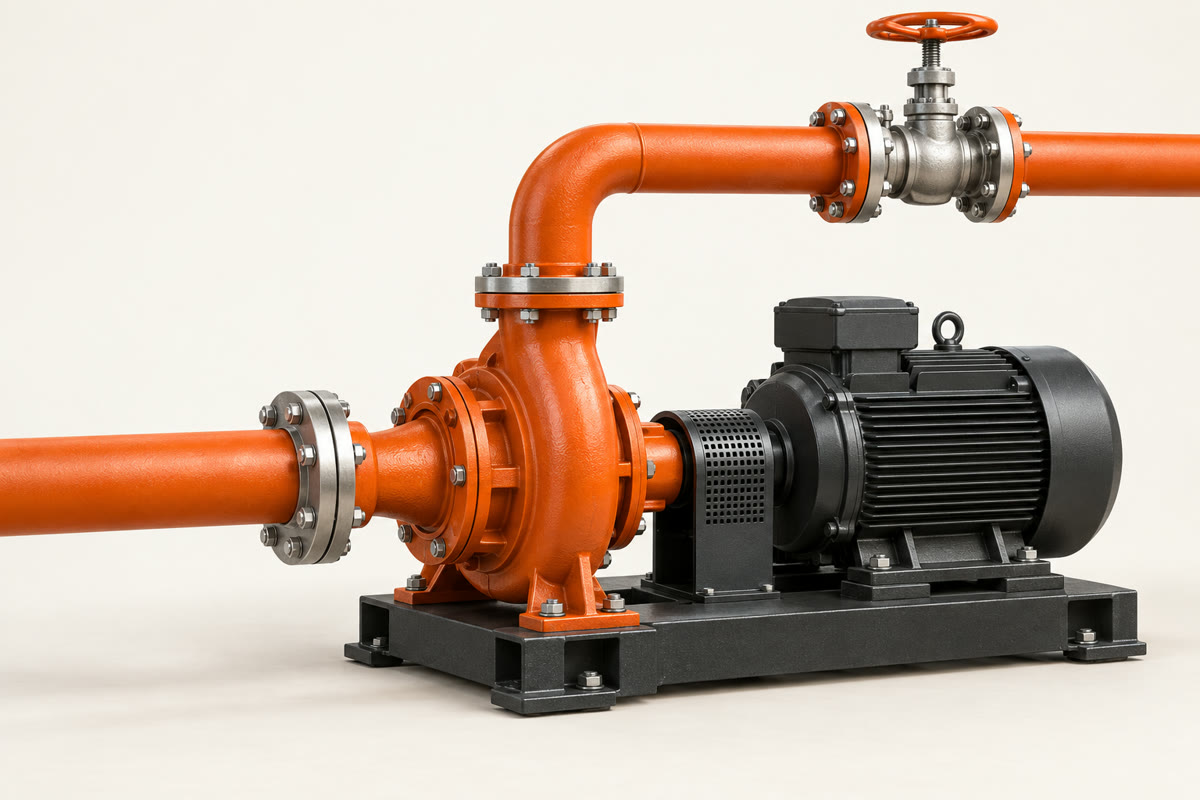
Try lowering the speed, adding valve resistance, or increasing static head. More throttling moves the operating point up and left. Lower speed moves it down the system curve. Enough static head can stop positive flow in this simplified model.

H_system = H_static + KQ²

Static head includes elevation and imposed pressure differences. Friction grows approximately with flow squared when the flow regime and resistance coefficients are suitable for that approximation. Real system curves can change with fluid properties, fouling and operating configuration.

What does the valve dissipate every hour?

Use the measured flow and head drop across the valve. The hydraulic loss is ρgQΔH. Dividing by the assumed pump and motor efficiencies gives an input-power equivalent, not guaranteed recoverable savings.

Hydraulic loss

Input equivalent

Hourly cost equivalent

Annual cost equivalent

The default example is hypothetical: water at 100 m³/h, a 20 m valve loss, 70% pump efficiency, 95% motor efficiency, $0.12/kWh, and 8,000 hours/year. It gives 5.45 kW dissipated hydraulically, 8.19 kW input equivalent, and about $7,865/year. Use your own currency consistently; the tariff is an editable assumption, not a quoted energy price.

A retrofit changes the duty point and efficiencies. Compare complete measured duty cycles, required head, minimum-flow limits, drive losses and installed cost before estimating actual savings. Valve position alone does not establish its pressure loss.

Twenty percent slower. Roughly half the power?

At corresponding operating points for the same impeller, the affinity relationships are Q ∝ N, H ∝ N² and shaft power ∝ N³, assuming similar efficiency. At 80% speed, 0.8³ = 0.512: about 51% of the reference power.

That is not a universal system savings formula. The estimate is most useful in friction-dominated systems with little static head. With substantial static head, flow does not fall in direct proportion to speed; the operating point and efficiency shift. Electrical input also depends on motor and drive efficiency.

The DOE tip sheet explicitly makes the low-static-head qualification. The video keeps “roughly” for this reason. The interactive chart deliberately lets you change static head to see where simple proportional thinking breaks down.

The source behind the shorthand.

The video's “one in five kilowatt-hours” refers to the 2001 Pump Life Cycle Costs guide's estimate of nearly 20% of global electrical-energy demand. It is historical context, not a newly measured 2026 statistic. The later variable-speed guide describes a motor-energy denominator; those wordings should not be treated as interchangeable.

A partially closed control valve may be necessary for process control. The video's 10%-shut example comes from the variable-speed guide; it is not a universal valve specification or a claim that 10% closure means 10% energy loss.

• Hydraulic Institute, Europump and US DOE: Variable Speed Pumping (2004). Pump/system intersections, throttling and limitations of speed control.
• US DOE: Control Strategies for Centrifugal Pumps with Variable Flow Rate Requirements (2007). Cube-law estimate, duty-cycle comparisons and efficiency qualifications.
• Hydraulic Institute, Europump and US DOE: Pump Life Cycle Costs (2001). Historical electricity estimate and whole-life cost approach.

Educational examples for centrifugal pumps. They are not a vendor curve, a pump selection, or operating instructions. Positive-displacement pumps behave differently. Check the manufacturer's operating envelope, NPSH requirements and application-specific constraints for real equipment.